IMPLEMENTATION OF THE EXPECTATION MAXIMIZATION ALGORITHM
Introduction
Nowadays biological research interests are quite focused in recognizing common patterns in cells responses, maybe as much as
in knowing specific points in cellular outcomes. The efforts being done are important because, by discovering pathways
shared among many cells, it can be possible to reach a better understanding of the mechanisms underlying cellular activity and this will
allow scientists to modify them.
Such common reactions in cells are normally linked to the presence of short elements or motifs
that have important roles in cells. These elements can be studied in two stages. First of all,
one can study motifs inside genes. Some genes might give the same answer to their environmental
conditions, which is often studied using techniques based on microarrays and computational
analysis. When a set of those genes that seem to be co-regulated is described, it is possible
to study their sequences promoters to find whether they have a common motif responsible for
that transcriptional activation. Secondly we can also look for similarities into protein
sequences, as many of them share functional regions (as signal peptides, phosphorilation sites, etc.) which can be studied too.
However, many times little or nothing is known about the motifs we are looking for, neither the structure
nor the situation. Moreover, these elements are normally quite short so they are easily hidden
among the long sequences surrounding them. Therefore, many motifs remain still to be discovered.
Different techniques are being used day by day in order to solve these problems.
For instance, we have talked about microarrays, but the best approaches seem to link with methods based on informatics, that
are already essential tools. Actually, computational systems open great expectations at discovering these hidden sequences.
Many programs have been developed over the past few years and are being improved each day.
Return to Index
Objectives
The aim of this project is to provide a mechanism to help finding new patterns related to genes’ or proteins’ activity, like
promoters or splicing sites for genes, or many functional domains for proteins.
In order to accomplish this, we have made a program based on the implementation of a well described algorithm already in use.
The Expectation-Maximization (EM) Algorithm, as it is called, appears to be a powerful tool, which works with a given set of
sequences and runs out a curl (iterative composition) to find inside the sequences the most probable motifs that may share a
common function in genes’ or proteins’ activity.
The importance of finding new motifs involves another crucial point. As it is known, genome regions that codify for an important
biologic function tend to maintain their DNA sequence quite constant. Therefore, if we are able to detect some evolutionary
maintained regions, those suspected motifs may have an unknown cellular function, which probably will be interesting
to discover.
Return to Index
The Program
What is the EM Algorithm?
The Expectation-Maximization (EM) Algorithm is an iterative method to estimate some unknown parameters given a set of data.
From the biological point of view, the EM algorithm can be implemented to search putative biological motifs in a set of sequences. Because the set of sequences is assumed to be a random sample from a random process, we cannot hope to definitively discover the real underlying parameter values. However, we can use statistical methods to arrive at good estimates. Then, instead of using local multiple alignment methods, the EM algorithm uses statistical modelling and *heuristics
to discover motifs by fitting a statistical model to de dataset of sequences.
One way of doing this is maximum likelihood estimate, which consists of finding the parameter values which maximize the likelihood of the model given the data. When the user provides the dataset of sequences, the algorithm fits the parameters of the model to the observed data (the sequences). After running the algorithm, it outputs the parameters of the motif component sequence of the sequence model. To choose the best model, EM uses a heuristic function based on the maximum likelihood ratio test.
The EM algorithm has three running possibilities, depending on the motifs you are searching:
- the OOPS model (from One Occurrence Per Sequence), that looks for one motif in each sequence;
- the ZOOPS model, that admits the possibility that some sequences have no motif (Zero occurrences);
- the TMC model, that permits the existence of a any number of non-overlapping motifs (from none to more than one).
In this website you will only be able to run the OOPS model.
*heuristic: an heuristic is a commonsense rule (or set of rules) intended to increase
the probability of solving some problem. It can also be considered as a way of directing your
attention fruitfully. return
The EM Algorithm step by step
The Input
The user of EM algorithm provides the dataset of sequences (DNA or protein sequences) and has to choose the estimation for the length of the motif he/she is searching.
The Steps
Given these sequences, the algorithm will try to create a probabilistic model, which has two components:
- the set of similar sub-sequences of fixed width (the motif),
- a description about the remaining positions in the sequences (the background).
To generate the probabilistic model we often construct an initial position weight matrix (PWM). The four rows of this matrix contain the four nucleotides (or 20 rows for 20 aminoacids); on the columns, the first one contains the information about the background and next columns refer each one to the positions of the motif.
1- Initialization
The first objective at the starting of the algorithm will be filling the matrix with the frequencies of each nucleotide or each aminoacid at the background and their frequencies at each particular position of the motif. As we have not analysed any sequence still, the PWM starts being full of 0s.
Then, the first step will consist of updating the matrix with the real values. To achieve this, we must decide where the motif begins and, as we probably have no idea at all, the first matrix is constructed taking a random initiation site for the motif in each one of the sequences we are analysing.
2- The E-Step (expectation)
In the E-step, the algorithm evaluates the goodness of the current model (that is, the last PWM calculated). The purpose is to calculate the probability that the motif starts in a particular position of the sequence for each sequence, evaluating the weight of each possible starting site.
To do this, the algorithm uses the current model (the PWM) and punctuates each candidate using the motif columns to score nucleotides or aminoacids belonging to the motif, and the background column to score the rest of them.
To get the final probability for each one, it is necessary to normalize (divide each score by the sum of all the other sites score) the obtained values to compare among starting points.
3- The M-Step (maximization)
In the M-step the algorithm will use the calculated probabilities in the E-step to update the model, to estimate the expected letters frequencies in the background positions and at each position in the motif occurrences. These expected letter frequencies constitute the next guess, the next model explained in the PWM, for the E-step.
In this step, the PWM is reinitialized to 0s, and the normalized scores for each candidate of each sequence will fill the frequency positions. The way of doing this is by analyzing each sequence and adding at every position of the matrix, the normalized score of each candidate.
When the algorithm completes the step, the result will be that the sites matching the model better will reinforce the distribution and will tend to remain in the model.
In the M-step we also calculate the log-likelihood of the model from the PWM, to make comparisons between models possible.
4- Finalization
The EM algorithm can be stopped in two ways.
The first one involves running the E and M-steps until the algorithm reaches the convergence. At each step, the algorithm compares the log-likelihood from the last model with the one it has just calculated. It will come a time when the difference between them will be low enough to consider that the result is not improving any more. This means that the algorithm has got to convergence and so it will stop running.
The other way depends on the user (although it is pre-established in our program). One may consider that a certain number of iterations are enough to consider that the model is quite good, and no more iterations need to be run. When the algorithm arrives at these rounds, it exits the iteration (in our program the rounds are 1000 iterations if convergence is not achieved before).
The Output – How should you consider your results?
The principal output is a series of probabilistic sequence models, each corresponding to one motif, whose parameters have been estimated by expectation maximization.
Concretely, after running the algorithm using the provided program in this website, the user gets:
- the log-likelihood of the current model,
- a list where the motifs found in each sequence appear aligned to permit a quick view of their similarity, accompanied of the score of each candidate,
- the information that each nucleotide or aminoacid represents at each position of the motif,
- the PWM for the accepted model (with the relative frequencies of the nucleotides or aminoacids in the background and in the positions along the motif),
To evaluate one’s results it has to be considered that:
- the log-likelihood of the model is a negative number because it represents de logarithm of a very little number (it is not rare to get a number similar to -10000). The reason for the likelihood to be so small is that the maximum number to be achieved is 1. As this is only the sum of the likelihood of all the possible models, the best likelihood remains still very small. Also, this number is very dependent on the length of the sequence because as it is longer, more possible models are allowed.
- the score for each candidate
- the information that contributes each position is expressed in bits of information. For nucleotides, the maximum information is 2 (as 2 is the exponent for a base of 2 to get 4, the four possibilities). For aminoacids, this number is proportional to the 20 aminoacids, that is, 4.32, calculated in the same way.
Testing the EM Algorithm
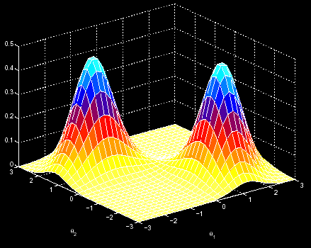
One may imagine the EM algorithm as a process localized in a 3D space. There we have the sequence to analyse, and the EM tries to find the point in that space with the highest probabilities of finding the common pattern in the sequences. In this movement along the 3D space, it is supposed that, at each iteration, we go up in the probability scale. However, this fact makes possible that, once we have began the analysis in a random point, we cannot reach the maximum probability point (the left one), but only arrive at a local maximum (the right one). Then, we might not acheive to find the motif (figure 1).
In order to avoid these cases we made 3 different implementations of the OOPS version. Here we describe the steps we made to get to the final program available on the website. In the “Results & Discussion” it is possible to take a look at the results we got.
We first implemented one program (the so called “OOPS”) based on the EM algorithm.
Afterwards, we tried two improvements. The first one consists of a previous step where 10 random starting points are tested and the initial matrix is keeped for each of them. The one that gives the highest log-likelihood after one E and M-step round is taken as the “random” initial position and the algorithm runs from that place. This program is being called “OOPS_2”.
Finally, the last update in OOPS_3 was done by changing the initial step. Instead of trying the multistart option, we tested a new strategy. In this case, a random sequence is divided in windows containing as much nucleotides (or aminoacids) as the motif length, and this window passes over the other sequences (sliding windows). The program punctuates how much matching symbols can be counted between each sliding window and each sequence fragment (the possible motifs in the other sequences). After passing all the possible windows from the chosen sequence along all the other sequences we will accept as the putative motif the window where more positions are equal in the other sequences. Therefore, the initial points with the best score in each sequence are used to construct the initial matrix. This way of acting is quite slow, proportionally to the sequence and motif lengths. However, from this starting point, the number of iterations need to be done before reaching convergence is really low.
If you want to see the programs code, click on the links.
OOPS
OOPS_2
OOPS_3
OOPS_proteins
RUN THE PROGRAM
Click here if you want to run the program!
Return to Index
Results & Discussion
To test the different versions of our program, we generated a dataset of sequences as a positive control. This file contains 4 random sequences with the TATATA motif, to assure that the program could easily unmask the pattern in the sequences.
After that, we ran the 3 programs 10 times each one with these sequences, calculating the mean likelihood achieved at the end (convergence). In the next figures a comparison of the results obtained is shown.
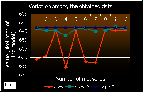
Figure 2 shows the fluctuation among the results obtained by each version. OOPS shows much more variation in the likelihood values than OOPS_2 and _3. This means that a random beginning of the EM algorithm probably converges at a local maximum. In OOPS_3 gets always the same correct result. So, the approach in this version leads the program to initiate the iterations near the maximum. OOPS_2 improvement also works well, but some times it gets a local maximum (that is dependent on the number of initialization processes and on the number of sequences and their length (data not shown)).
|
|
|
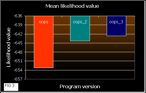
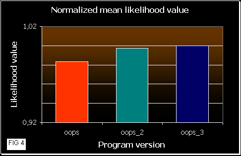
In figure 3 we can see how good the programs are. As higher is the mean likelihood values, the program works better (it gets better results more times). OOPS_3 reaches the best results, quite similar to OOPS_2, and OOPS shows poorer values, as we would expect. As mean likelihood depends on the sequence length, we also normalized the values in figure 4.
A que te gusta muxo muxo??? 
Return to Index